
Intro
To kick off this article, I’d like to explain the interpretability of a machine learning (ML) model.
According to Merriam-Webster, interpretability describes the process of making something plain or understandable. In the context of ML, interpretability provides us with an understandable explanation of how a model behaves. Basically, it helps us figure out what’s behind model predictions and how these models work. Miller and Tim’s “Explanation in Artificial Intelligence: Insights from the Social Sciences” states that “Interpretability is the degree to which a human can understand the cause of a decision.” By utilizing ML interpretability methods, we increase this degree and allow humans to consistently predict the model’s behavior.
Moreover, fairness and unbiasedness have recently become important auxiliary criteria for model optimization. ML interpretability is an essential tool to check these properties for ML systems.
In this work, I’ll let you in on major methods of tackling the interpretability of ML models using Python and explain how to build a resilient machine learning infrastructure that serves as a foundation for artificial intelligence, accelerating the time to market for AI-powered projects.
[Related Article: Not Always a Black Box: Machine Learning Approaches For Model Explainability]
Classes of Interpretability Methods
According to Christoph Molnar, author of the amazing “Interpretable Machine Learning”, all methods of ML interpretability can be broken down into the following classes:
Relative to the moment the interpretation task was set
First, the methods of interpretability can be classified relative to the moment a data scientist decides to interpret a model:
- Ante Hoc. The model’s interpretability is a required criterion for selecting an ML model. It’s also called “intrinsic,” since the selected model includes a natural way of interpretation based on the internal working of that particular learning algorithm. This mindset is more inherent to econometrics than ML.
- Post Hoc. ****Interpretation is an additional bonus, required when the model is already ready for use.
The first type of methods is reduced to solving problems using relatively simple models whose structure is easy to interpret—sparse linear models, logistic regression, or a single decision tree. The second type of method is suitable when a ready-to-use model needs interpretation.
Model-Specific vs. Model-Agnostic
Secondly, methods of interpretability can also be broken down based on their area
of application:
- Model-specific. The methods of this group depend on the type of selected model. For instance, methods that use gradient values in neural networks can be applied exclusively to neural networks and methods which use splits in tree-based models cannot be applied to other methods.
- Model-agnostic. The methods of this group treat predictive models as black-box and place no assumptions on the internal structure of the model.
Scope
Lastly, interpretation methods can also have a different scope of interpretation—they’re capable of explaining either a single prediction made by a model or they can explain an entire model’s behavior. The first option is called local and the latter is global. The local scope is usually called the instance/sample/prediction explanation and the global scope is usually called the model explanation.
However, the scope can also be somewhere in the middle, explaining not a single prediction, but a group of them, while leaving the behavior of a global model out of scope.
Achieving a global interpretation of the explained model is an extremely complex task, even for algorithms with a high intrinsic capacity for interpretability, like linear models. For instance, explaining the full scope of behavior of a linear model with 20 parameters would require imagining a hyperplane in 20 dimensions! Thus, global interpretation requires not only an interpretable model, but also careful feature engineering. This approach is typical for econometrics and ad hoc interpretability. In ML, most of the research focuses on explaining local model behavior understanding that it’s more feasible for humans. Further, in this article, we’ll focus on model agnostic, local, and post hoc interpretability methods.
Methods
Partial Dependency Plot
One of the simplest and most understandable methods is a partial dependency graph. This dependency graph shows us the dependency of a target variable from a particular feature. We plot feature values on one axis, from min to max, and we plot an aggregated target variable values on another axis. Since we account only for a few features in our analysis, higher order interactions will be missed. It’s a good heuristic to select features for an analysis by **feature_importance** values obtained from a classifier.
Here’s one example of getting a PD plot from the sklearn library.
# Example on PD plot in sklearn library
from sklearn.ensemble.partial_dependence import partial_dependence, plot_partial_dependence
X_train, X_test, y_train, y_test = train_test_split(...)
clf = Regressor(...)
clf.fit(X_train, y_train)
features = [0, 1, (0, 1)]  # Features used for computing and plotting PDPlot
fig, axs = plot_partial_dependence(clf, X_train, features)
plt.show()

➕ Pros:
- Easy and intuitive
- Available in sklearn
➖ Cons:
- Assumption of feature independence
- Loss of higher-order interactions
Since we aggregate the target variable, we will lose any heterogeneous trends in data. For example, imagine, a group of patients, half of which smoke. The smokers have a higher cancer probability with age, but the nonsmokers have a lower cancer probability prediction with age. These two trends, if aggregated, would diminish each other.
Permutation Importance
Permutation Importance is an intuitive way to assess the impact of a feature on the black-box model performance. The algorithm idea starts developing from the intuition that each feature has made some impact on the value of the loss function of the explained algorithm and that removing this feature will result in a different loss score. Therefore, the simplest way to assess the impact of the feature on the target loss would be to remove it from the original dataset and reevaluate loss.
However, this will require retraining for almost all models, since most of them operate with a static, predefined shape of input, and dropping this feature will change the shape of the input. This approach isn’t practical—model retraining can take a long time. Instead of this, we can perform a clever trick: replace the values of this feature with random noise, so it will lose the relationship with the target value. This will have almost the same effect as removing this feature from the dataset. Since the noise has to be from the same distribution as the original feature, we will simply shuffle this feature column to produce the desired noise.
Here’s an example of this algorithm from the eli5 library on the cervical cancer dataset.
from eli5.sklearn import PermutationImportance
import sklearn

X_train, X_test, y_train, y_test = train_test_split(...)
model = sklearn.some_model().fit(X_train, y_train)
perm = PermutationImportance(model).fit(X_test, y_test)
eli5.show_weights(perm)

Since we shuffle our data to get the noise, the calculated feature importances can differ depending on shuffle and random seed. To mitigate this, we calculate feature importance multiple times and present the distribution of feature importances in the form of mean and confidence intervals.
➕ Pros:
- Simple and intuitive
- Available through the eli5 library
- Easy to compute
➖ Cons:
- Requires labeled test data to compute the loss
- Different shuffles may give different results
- Greatly influenced by correlated features
SHAP
SHAP is a library unifying multiple interpretability methods under the concept of Shapley values. A Shapley value is a concept from game theory, basically a unique distribution (among the players) of the total surplus generated by a coalition of all players in a cooperative game. In other words, a Shapley value is a value which demonstrates to each player how important they are to overall cooperation and what payoff they can reasonably expect. At first glance, the idea seems strange and unrelated to the concept of interpretability, but really it’s not. If we think of every feature as a player, the sample as their coalition, and the score function as the worth of this coalition, then the Shapley value for each feature will show how that particular feature impacts the final score.
To evaluate such a value for a particular sample, we need to evaluate all possible coalitions of feature values with and without this feature. As you can imagine, the number of possible coalitions exponentially increases with the number of features, so calculating the exact solution isn’t an option. SHAP unifies multiple interpretability methods under its hood to overcome the problem of calculating exact Shapley values. SHAP offers multiple algorithms to calculate so-called SHAP values which have the same desirable properties as the Shapley values. One such algorithm is the TreeExplainer, which computes the explanations for tree-based models, whether it’s XGboost, LightGBM, CatBoost, or scikit-learn models. It’s much faster than the naive method of evaluating all possible coalitions.
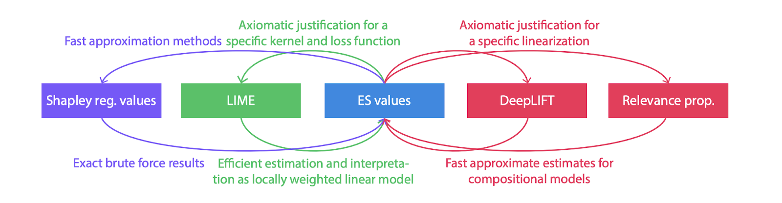
Methods unified under concept of SHAP
Here is the example of TreeExplainer on Boston house pricing dataset:
import shap

# load JS visualization code to notebook
shap.initjs()

# train XGBoost model
X,y = shap.datasets.boston()
model = xgboost.train(...)

# explain the model's predictions using SHAP values
# (same syntax works for LightGBM, CatBoost, and scikit-learn models)
explainer = shap.TreeExplainer(model)
shap_values = explainer.shap_values(X)

# visualize the first prediction's explanation (use matplotlib=True to avoid Javascript)
shap.force_plot(explainer.expected_value, shap_values[0,:], X.iloc[0,:])

For interpreting black boxes, SHAP provides the KernelExplainer class. For more details on SHAP, refer to their repository.
➕ Pros:
- We can see both features pushing predictions up and down
- Based on solid theory. SHAP values have useful and proven mathematical properties
- TreeExplainer is fast
➖ Cons:
- The inclusion of unrealistic data instances
- Computationally expensive in the general case case
- Based on solid theory. It can be hard to dive into all the math inside this method
LIME
LIME is one of the most popular libraries, with over 5K stars at Github. It’s based on the method of the same name described in “’Why Should I Trust You?’: Explaining the Predictions of Any Classifier” delivered at the Association for Computing Machinery in 2016. This method is model-agnostic and intended to explain the local behavior of the model around some point X.
It’s important to point out that LIME assumes that the local model behavior is far less complex than the global one. If this assumption is true, we can approximate the local behavior with a less complex, more interpretable model. We call such models “local surrogates,” since they approximate the local decision boundary of a black-box classifier.
To produce an explanation, LIME takes the vicinity of a particular instance and augments this instance so that we get more data in the local area around this instance. Next, the sparse linear model is trained on these nearby points. Since this model is interpretable, we can also interpret the local behavior around X. We can gradually reduce or increase the regularization factor in the linear model until we reach a suitable amount of nonzero coefficients.

There is one uncertainty about this algorithm: what does the “vicinity” of explained instance mean? These vicinity weights are calculated as its distance to X using a kernel function, an RBF kernel by default; instances closer to X are assigned a higher importance. However, picking the kernel width, the hyperparameter of kernel function, requires attention, because we can’t select the same kernel width for all cases. Here is the link to a discussion on how to select a proper kernel width. Still, even if we know the kernel width, we do not exactly know where this explanation applies. The explanations that are produced are local and not applicable everywhere. The range of applicability is called coverage. It would be good to assess the coverage of the explanations.
Here is an example based on the adult dataset from the lime library developed by the authors of the method.
import lime
import sklearn

data = # load adult dataset

categorical_features = [1,3,5,6,7,8,9,13]
categorical_names = {}
for feature in categorical_features:
    le = sklearn.preprocessing.LabelEncoder()
    le.fit(data[:, feature])
    data[:, feature] = le.transform(data[:, feature])
    categorical_names[feature] = le.classes_

X_train, X_test, y_train, y_test = train_test_split(data)

rf = sklearn.ensemble.RandomForestClassifier().fit(X_train, y_train)
explainer = lime.lime_tabular.LimeTabularExplainer(X_test,
																									 feature_names = feature_names,
																									 class_names=class_names,
                                                   categorical_features=categorical_features,
                                                   categorical_names=categorical_names,
																									 kernel_width=3)

exp = explainer.explain_instance(test[0], rf.predict, num_features=5)
exp.show_in_notebook(show_all=False)

For more details on LIME refer to their repository.
➕ Pros:
- Completely model-agnostic
- Plenty of contributors
➖ Cons:
- The inclusion of unrealistic data instances
- Ambiguity of how to select kernel width
- Unclear coverage
Anchor
The creators of LIME are active in the space of the interpretability of ML models. In 2018, two years after the original article about the LIME method was published, they revealed a study called “Anchors: High-Precision Model-Agnostic Explanations” at the AAAI event in the Human-Computer Interaction section. The authors introduced a novel model-agnostic system that explained the behavior of complex models with high-precision rules called anchors, representing local, “sufficient” conditions for predictions.
It’s important to bear in mind the reasons that the creators of this highly popular library published a new, follow-up paper. In the Anchor paper, M.T. Ribeiro et al. suggested that it was unclear how to assess the coverage of locally accurate interpretations produced by local surrogates. They provided insights into the model behavior, but the same explanations couldn’t be used outside the local vicinity of the explained sample, and the scope of local vicinity wasn’t really clear. If this scope is not clear, the explanation can be misused outside of this scope and will most likely result in an invalid conclusion. To overcome the aforementioned problem, Ribeiro et al. designed a new method they called Anchor. They asked a group of 26 students who had been studying ML to make predictions about novel samples given explanations produced by LIME and Anchor on another part of the same dataset. Anchor showed higher accuracy and comprehensibility than the LIME method, resulting in a lower time per prediction. But what is the Anchor method? Essentially, it generates explanations called “anchors.” These anchors are part of the explained sample anchoring it to a specific label produced by the model for this explained sample. Basically, each anchor is a set of predicates called A present in the explained sample. These predicates can be in any form and generally depend on the type of data being explained. The set of predicates is called an anchor if it anchors the sample to a label. In other words, if we change the sample in many different ways according to some perturbation distribution, which we’ll call D, without breaking the predicates, and the label doesn’t change, then we have found our anchor.

The ratio of the number of times when the label hasn’t changed after perturbations to the number of all samples satisfying the anchor is called the precision of this anchor. The precision directly reflects the quality of the anchor; it shows how stable the anchor is to perturbations. The exact definition of the precision is

Since estimating the expected value of this distribution is intractable for most of the problems, probabilistic definition is introduced:

This probabilistic precision is used throughout the method, with tau being the precision threshold and sigma being the possibility of missing this threshold. However, precision isn’t the only metric we want to optimize. High precision is a sufficient condition to call a set of predicates an anchor, but we can generate multiple anchors for a single explanation. In that case, we’d consider the most representative anchor or the anchor with the highest coverage. Coverage is the probability that this anchor will be present in other samples. This property can be directly seen as the measure of the scope covered by an explanation.

Therefore, if multiple anchors describe a prediction, the most global one is selected. It’s important to note that coverage is the second metric and that the predictions should already be sufficient for the high-precision requirement.

Thus, the anchor search should be formulated as a combinatorial optimization problem of maximization coverage of a set of predicates with regards to the high-precision requirement.


To construct these anchors, the authors propose a bottom-up construction of anchors in one of two ways: greedy or beam-search. Bottom-up construction means that we construct a set of predicates gradually, adding them one by one, until a condition based on precision and coverage isn’t satisfied.
The algorithm can be considered computationally expensive, since evaluating the precision of each candidate explanation requires calling a prediction function on data sampled from ***D(z|A)***.
To mitigate these costs, the authors propose considering each candidate set A as an arm with a Bernoulli distributed reward in a multi-armed bandit. This Bernoulli distribution has parameter p equal to the precision of the anchor.

To solve this multi-armed bandit problem, the KL-_LUCB algorithm is used. This algorithm takes the pool of anchors and “pulls” each anchor in special way to learn the p of the Bernoulli distribution in the least number of pulls. Each pull evaluates a batch of perturbed data and returns the precision calculated on this batch. After the KL-LUCB algorithm is called, it returns either the best set of anchors or just the best anchor from the current pool of anchors, depending on whether a greedy or beam search is used. If multiple returned anchors satisfy the precision requirements, the best anchor is determined by the coverage.
Unfortunately, this library is not fully ready, but there are a few notebooks available to see how the method works in the authors GitHub repository.
Here is an example of explanations produced by this method on an adult dataset.
Anchor = ['Capital Gain == None',
 'Sex ==  Male',
 'Occupation == Blue-Collar',
 'Capital Loss == None',
 'Hours per week < 84.0',
 'Age < 63.0']

Coverage = 0.081
Precision = 0.982
For more details on Anchor refer to their repository.
➕ Pros:
- Clear coverage
- Guaranteed high precision
- The anchors themselves are very expressive
➖ Cons:
- The inclusion of unrealistic data instances
- The code available in the original repository is still in progress
Conclusions
[Related Article: Redefining Robotics: Next Generation Warehouses]
In this article, I have tried to explain the key methods associated with model-agnostic interpretation. We have discussed the pros and cons of methods such as LIME, Anchor, SHAP, PDP, and MDA. Currently, I’m implementing these methods on a range of ML projects for Silicon Valley tech companies as a part of the Provectus AI consultancy. Check some of the hottest projects that I’m really proud of here.
If you have any questions or suggestions, please leave a comment or reach out to me on Twitter or via email at ygavrilin@provectus.com
Originally Posted Here
