
Con un modelo de machine learning se puede crear un algoritmo que es capaz de detectar y reconocer el género de un individuo sólo por el tono de su voz usando Tensorflow en Python.
Gender recognition by voice es una técnica en la que permite determinar la categoría de género de un hablante mediante el procesamiento su voz, en este tutorial, trataremos de clasificar el género por la voz utilizando el marco de TensorFlow en Python.
El reconocimiento de género puede ser útil en muchos ámbitos, incluido el reconocimiento automático del habla, en el que puede ayudar a mejorar el rendimiento de los sistemas. También puede utilizarse para clasificar las llamadas por género, o puede añadirse como una característica a un asistente virtual que sea capaz de distinguir el género del hablante.
Los pasos que se deben realizar para llevar a cabo este proceso son:
- Preparación del conjunto de datos
- Entrenando el modelo
- Test del modelo
- Prueba del modelo con nuestra propia voz
A continuación se muestra el código completo con sus pasos:
To get started, install the following libraries using pip:
To follow along, open up a new notebook and import the modules we gonna need:
import pandas as pd
import numpy as np
import os
import tqdm
from tensorflow.keras.models import Sequential
from tensorflow.keras.layers import Dense, LSTM, Dropout
from tensorflow.keras.callbacks import ModelCheckpoint, TensorBoard, EarlyStopping
from sklearn.model_selection import train_test_split
Now to get the gender of each sample, there is a CSV metadata file (check it here) that links each audio sample’s file path to its appropriate gender:
df = pd.read_csv("balanced-all.csv")
df.head()
Here is how it looks like:
                                filename  gender
0  data/cv-other-train/sample-069205.npy  female
1  data/cv-valid-train/sample-063134.npy  female
2  data/cv-other-train/sample-080873.npy  female
3  data/cv-other-train/sample-105595.npy  female
4  data/cv-valid-train/sample-144613.npy  female
Let’s see how the dataframe ends:
df.tail()
Output:
                                    filename gender
66933  data/cv-valid-train/sample-171098.npy   male
66934  data/cv-other-train/sample-022864.npy   male
66935  data/cv-valid-train/sample-080933.npy   male
66936  data/cv-other-train/sample-012026.npy   male
66937  data/cv-other-train/sample-013841.npy   male
Let’s see the number of samples of each gender:
# get total samples
n_samples = len(df)
# get total male samples
n_male_samples = len(df[df['gender'] == 'male'])
# get total female samples
n_female_samples = len(df[df['gender'] == 'female'])
print("Total samples:", n_samples)
print("Total male samples:", n_male_samples)
print("Total female samples:", n_female_samples)
Output:
Total samples: 66938
Total male samples: 33469
Total female samples: 33469
Perfect, a large number of balanced audio samples, the following function loads all the files into a single array, we don’t need any generation mechanism as it fits the memory (since each audio sample is only the extracted feature with the size of 1KB):
def load_data(vector_length=128):
    """A function to load gender recognition dataset from `data` folder
    After the second run, this will load from results/features.npy and results/labels.npy files
    as it is much faster!"""
    # make sure results folder exists
    if not os.path.isdir("results"):
        os.mkdir("results")
    # if features & labels already loaded individually and bundled, load them from there instead
    if os.path.isfile("results/features.npy") and os.path.isfile("results/labels.npy"):
        X = np.load("results/features.npy")
        y = np.load("results/labels.npy")
        return X, y
    # read dataframe
    df = pd.read_csv("balanced-all.csv")
    # get total samples
    n_samples = len(df)
    # get total male samples
    n_male_samples = len(df[df['gender'] == 'male'])
    # get total female samples
    n_female_samples = len(df[df['gender'] == 'female'])
    print("Total samples:", n_samples)
    print("Total male samples:", n_male_samples)
    print("Total female samples:", n_female_samples)
    # initialize an empty array for all audio features
    X = np.zeros((n_samples, vector_length))
    # initialize an empty array for all audio labels (1 for male and 0 for female)
    y = np.zeros((n_samples, 1))
    for i, (filename, gender) in tqdm.tqdm(enumerate(zip(df['filename'], df['gender'])), "Loading data", total=n_samples):
        features = np.load(filename)
        X[i] = features
        y[i] = label2int[gender]
    # save the audio features and labels into files
    # so we won't load each one of them next run
    np.save("results/features", X)
    np.save("results/labels", y)
    return X, y
The above function is responsible for reading that CSV file and loading all audio samples in a single array, this will take some time the first time you run it, but it will save that bundled array in results folder, which will save us time in the second run.
Now this is a single array, but we need to split our dataset into training, testing and validation sets, the below function is doing that:
def split_data(X, y, test_size=0.1, valid_size=0.1):
    # split training set and testing set
    X_train, X_test, y_train, y_test = train_test_split(X, y, test_size=test_size, random_state=7)
    # split training set and validation set
    X_train, X_valid, y_train, y_valid = train_test_split(X_train, y_train, test_size=valid_size, random_state=7)
    # return a dictionary of values
    return {
        "X_train": X_train,
        "X_valid": X_valid,
        "X_test": X_test,
        "y_train": y_train,
        "y_valid": y_valid,
        "y_test": y_test
    }
We’re using sklearn‘s train_test_split() convenient function, which will shuffle our dataset and splits it into training and testing sets, we then run it again on training set to get the validation set. Let’s use these functions:
# load the dataset
X, y = load_data()
# split the data into training, validation and testing sets
data = split_data(X, y, test_size=0.1, valid_size=0.1)
Now this data dictionary contains everything we need to fit our model, let’s build the model then!
Building the Model
For this tutorial, we are going to use a deep feed-forward neural network with 5 hidden layers, it isn’t the perfect architecture, but it does the job so far:
def create_model(vector_length=128):
    """5 hidden dense layers from 256 units to 64, not the best model."""
    model = Sequential()
    model.add(Dense(256, input_shape=(vector_length,)))
    model.add(Dropout(0.3))
    model.add(Dense(256, activation="relu"))
    model.add(Dropout(0.3))
    model.add(Dense(128, activation="relu"))
    model.add(Dropout(0.3))
    model.add(Dense(128, activation="relu"))
    model.add(Dropout(0.3))
    model.add(Dense(64, activation="relu"))
    model.add(Dropout(0.3))
    # one output neuron with sigmoid activation function, 0 means female, 1 means male
    model.add(Dense(1, activation="sigmoid"))
    # using binary crossentropy as it's male/female classification (binary)
    model.compile(loss="binary_crossentropy", metrics=["accuracy"], optimizer="adam")
    # print summary of the model
    model.summary()
    return model
We’re using a 30% dropout rate after each fully connected layer, this type of regularization will hopefully prevent overfitting on the training dataset.
An important thing to note here is we’re using a single output unit (neuron) with a sigmoid activation function in the output layer, the model will output the scalar 1 (or close to it) when the audio’s speaker is a male, and female when it’s closer to 0.
Also, we’re using binary cross entropy as the loss function, as it is a special case of categorical cross entropy when we only have 2 classes to predict. Let’s use this function to build our model:
# construct the model
model = create_model()
Training the Model
Now that we have built the model, let’s train it using the previously loaded dataset:
# use tensorboard to view metrics
tensorboard = TensorBoard(log_dir="logs")
# define early stopping to stop training after 5 epochs of not improving
early_stopping = EarlyStopping(mode="min", patience=5, restore_best_weights=True)

batch_size = 64
epochs = 100
# train the model using the training set and validating using validation set
model.fit(data["X_train"], data["y_train"], epochs=epochs, batch_size=batch_size, validation_data=(data["X_valid"], data["y_valid"]),
          callbacks=[tensorboard, early_stopping])
We defined two callbacks that will get executed after the end of each epoch:
- The first is the tensorboard, we gonna use it to see how the model goes during the training in terms of loss and accuracy.
- The second callback is early stopping, this will stop the training when the model stops improving, I’ve specified a patience of 5, which means it will stop training after 5 epochs of not improving, setting
restore_best_weightstoTruewill restore the optimal weights that was recorded during the training and assign it to the model weights.
Let’s save this model:
# save the model to a file
model.save("results/model.h5")
Here is my output:
Model: "sequential"
_________________________________________________________________
Layer (type)                 Output Shape              Param #
=================================================================
dense (Dense)                (None, 256)               33024
_________________________________________________________________
dropout (Dropout)            (None, 256)               0
_________________________________________________________________
dense_1 (Dense)              (None, 256)               65792
_________________________________________________________________
dropout_1 (Dropout)          (None, 256)               0
_________________________________________________________________
dense_2 (Dense)              (None, 128)               32896
_________________________________________________________________
dropout_2 (Dropout)          (None, 128)               0
_________________________________________________________________
dense_3 (Dense)              (None, 128)               16512
_________________________________________________________________
dropout_3 (Dropout)          (None, 128)               0
_________________________________________________________________
dense_4 (Dense)              (None, 64)                8256
_________________________________________________________________
dropout_4 (Dropout)          (None, 64)                0
_________________________________________________________________
dense_5 (Dense)              (None, 1)                 65
=================================================================
Total params: 156,545
Trainable params: 156,545
Non-trainable params: 0
_________________________________________________________________
Train on 54219 samples, validate on 6025 samples
Epoch 1/100
54219/54219 [==============================] - 8s 143us/sample - loss: 0.5514 - accuracy: 0.7651 - val_loss: 0.3807 - val_accuracy: 0.8508
Epoch 2/100
54219/54219 [==============================] - 5s 93us/sample - loss: 0.4159 - accuracy: 0.8326 - val_loss: 0.3464 - val_accuracy: 0.8536
Epoch 3/100
54219/54219 [==============================] - 5s 93us/sample - loss: 0.3860 - accuracy: 0.8466 - val_loss: 0.3112 - val_accuracy: 0.8744
<..SNIPPED..>
Epoch 16/100
54219/54219 [==============================] - 5s 96us/sample - loss: 0.2864 - accuracy: 0.8936 - val_loss: 0.2387 - val_accuracy: 0.9087
Epoch 17/100
54219/54219 [==============================] - 5s 95us/sample - loss: 0.2824 - accuracy: 0.8945 - val_loss: 0.2464 - val_accuracy: 0.9110
Epoch 18/100
54219/54219 [==============================] - 6s 103us/sample - loss: 0.2887 - accuracy: 0.8920 - val_loss: 0.2406 - val_accuracy: 0.9074
Epoch 19/100
54219/54219 [==============================] - 5s 95us/sample - loss: 0.2822 - accuracy: 0.8939 - val_loss: 0.2435 - val_accuracy: 0.9080
Epoch 20/100
54219/54219 [==============================] - 5s 96us/sample - loss: 0.2813 - accuracy: 0.8957 - val_loss: 0.2567 - val_accuracy: 0.8993
Epoch 21/100
54219/54219 [==============================] - 5s 89us/sample - loss: 0.2759 - accuracy: 0.8962 - val_loss: 0.2442 - val_accuracy: 0.9112
As you can see, the model training stopped at epoch 21, and reached about 0.2387 loss and almost 91% validation accuracy (this was on epoch 16).
Testing the Model
Since the model now is trained and the weights are optimal, let’s test it using our testing set we created earlier:
# evaluating the model using the testing set
print(f"Evaluating the model using {len(data['X_test'])} samples...")
loss, accuracy = model.evaluate(data["X_test"], data["y_test"], verbose=0)
print(f"Loss: {loss:.4f}")
print(f"Accuracy: {accuracy*100:.2f}%")
Check this out:
Evaluating the model using 6694 samples...
Loss: 0.2405
Accuracy: 90.95%
Amazing, we’ve reached 91% accuracy on samples that the model never seen before! That is great!
If you open up tensorboard (using the command: tensorboard --logdir="logs"), you’ll see loss and accuracy curves similar to this:
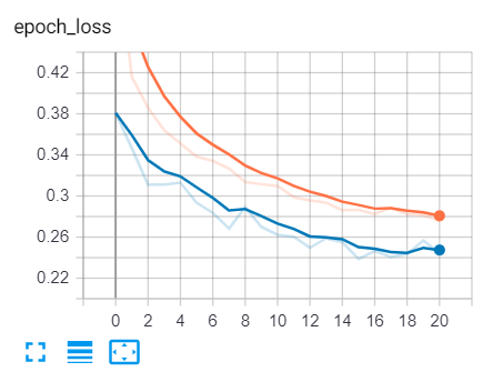
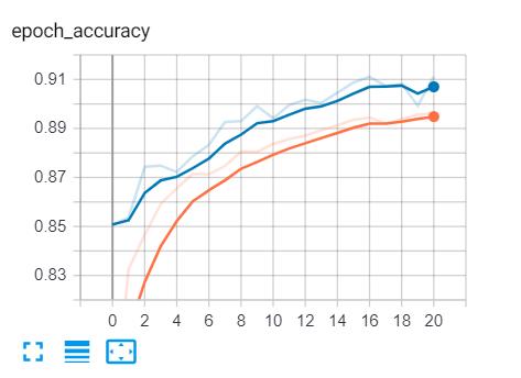
The blue curve is the validation set, whereas the orange is training set, you can see the loss is decreasing over time and the accuracy is increasing, that’s exactly what we expected!
Testing the Model with your own Voice
I know this is the exciting part, I’ve made a script that records your voice until you stop speaking (you can speak in any language though) and save it to a file, then extract features from that audio and feed it to the model to retrieve results:
import librosa
import numpy as np

def extract_feature(file_name, **kwargs):
    """
    Extract feature from audio file `file_name`
        Features supported:
            - MFCC (mfcc)
            - Chroma (chroma)
            - MEL Spectrogram Frequency (mel)
            - Contrast (contrast)
            - Tonnetz (tonnetz)
        e.g:
        `features = extract_feature(path, mel=True, mfcc=True)`
    """
    mfcc = kwargs.get("mfcc")
    chroma = kwargs.get("chroma")
    mel = kwargs.get("mel")
    contrast = kwargs.get("contrast")
    tonnetz = kwargs.get("tonnetz")
    X, sample_rate = librosa.core.load(file_name)
    if chroma or contrast:
        stft = np.abs(librosa.stft(X))
    result = np.array([])
    if mfcc:
        mfccs = np.mean(librosa.feature.mfcc(y=X, sr=sample_rate, n_mfcc=40).T, axis=0)
        result = np.hstack((result, mfccs))
    if chroma:
        chroma = np.mean(librosa.feature.chroma_stft(S=stft, sr=sample_rate).T,axis=0)
        result = np.hstack((result, chroma))
    if mel:
        mel = np.mean(librosa.feature.melspectrogram(X, sr=sample_rate).T,axis=0)
        result = np.hstack((result, mel))
    if contrast:
        contrast = np.mean(librosa.feature.spectral_contrast(S=stft, sr=sample_rate).T,axis=0)
        result = np.hstack((result, contrast))
    if tonnetz:
        tonnetz = np.mean(librosa.feature.tonnetz(y=librosa.effects.harmonic(X), sr=sample_rate).T,axis=0)
        result = np.hstack((result, tonnetz))
    return result
The above function is the function that is responsible for loading the audio file and extracting features from it, the below lines of code will use argparse module to parse an audio file path passed from the command line and make inference on it:
import argparse
parser = argparse.ArgumentParser(description="""Gender recognition script, this will load the model you trained,
                                    and perform inference on a sample you provide (either using your voice or a file)""")
parser.add_argument("-f", "--file", help="The path to the file, preferred to be in WAV format")
args = parser.parse_args()
file = args.file
# construct the model
model = create_model()
# load the saved/trained weights
model.load_weights("results/model.h5")
if not file or not os.path.isfile(file):
    # if file not provided, or it doesn't exist, use your voice
    print("Please talk")
    # put the file name here
    file = "test.wav"
    # record the file (start talking)
    record_to_file(file)
# extract features and reshape it
features = extract_feature(file, mel=True).reshape(1, -1)
# predict the gender!
male_prob = model.predict(features)[0][0]
female_prob = 1 - male_prob
gender = "male" if male_prob > female_prob else "female"
# show the result!
print("Result:", gender)
print(f"Probabilities::: Male: {male_prob*100:.2f}%    Female: {female_prob*100:.2f}%")
This won’t work if you execute it, as record_to_file() method isn’t defined (you can check the full script code here), but this helps me explain the code.
We’re using argparse module to parse the file path passed from command lines, if the file isn’t passed (using --file or -f parameter), the script will start recording using your default microphone.
We then create the model and load the optimal weights we trained before, and then we extract the features of that audio file passed (or recorded) and we use model.predict() to get the resulting predictions, here is an example:
$ python test.py --file "test-samples/16-122828-0002.wav"
Output:
Result: female
Probabilities:     Male: 20.77%    Female: 79.23%
And indeed, that sample that was grabbed from LibriSpeech dataset is a female! Again, get the code here.
Related: How to Play and Record Audio in Python
Conclusion
Now you have a lot of options to further make the model more accurate, one is trying to come up with another model architecture, you can also use Convolution or recurrent nets and see the results! I can expect you reach more than 95% accuracy, if you did so, please don’t hesitate to share it with us in the comments below!
You can also download the original dataset from Kaggle and use another feature extraction technique such as MFCC using the provided extract_feature() function, and then you can compare the results.
The whole tutorial material is located in this repository, check it out!
Finally, there is a similar tutorial in which you’ll learn how to recognize emotions from speech as well, check it out!
Learn also: How to Convert Text to Speech in Python
Para más información puede ver el post completo del autor AQUI
